Unique Risk Series – Article 2 out of 3
– Diversification
– Minimum Variance Portfolio
– Market Portfolio
In the first article of the Unique Risk series, we saw how portfolio diversification can help you achieve higher returns without necessarily exposing you to more risk.
We concluded that it is not the riskiness of an individual stock that matters, it’s actually how the stock affects the riskiness of your entire portfolio that determines whether you should invest or not.
In this article, I will describe what a minimum variance portfolio is and will show how investing in a minimum variance portfolio allows you to maximize the benefits of diversification.
Example
Let’s revisit the example used in the last article…
You are currently 100% invested in Stock A, which has an expected return of 4% and a standard deviation of 6%.
Since Stock B is negatively correlated to Stock A and has a higher expected return, we determined it was beneficial to invest in Stock B so we decided to invest 50% of the portfolio in Stock A and 50% of the portfolio in Stock B. This combination produced a portfolio with an expected return of 6% and a standard deviation of 5.81%.
We’re happy that we increased the expected return and lowered the standard deviation by investing in Stock B but is this 50/50 portfolio optimal?
Let’s find out!
Graph
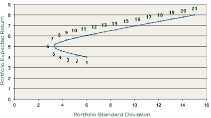
The following graph shows the expected return and standard deviation of different portfolios invested in varying amounts of Stock A and Stock B.
Each consecutive dot on the line represents a 5% increase in the amount of the portfolio invested in Stock B. For instance, dot 1 represents a portfolio invested 100% in Stock A and 0% in Stock B, dot 2 represents a portfolio invested in 95% in Stock A and 5% in Stock B, and so on until you reach dot 21, which represents a portfolio invested 0% in Stock A and 100% in Stock B.

You can see from the graph that it doesn’t make sense to invest in the portfolios represented by dots 1, 2, 3, 4, or 5 because you’d achieve a higher return while maintaining roughly the same standard deviation if you instead invested in 11, 10, 9, 8, or 7, respectively.
The portfolios represented by dots 6 through 21 are considered “efficient” because for those portfolios, it is not possible to obtain a higher expected return without also increasing the standard deviation.
Looking at this graph, it is easy to see which portfolio is the minimum variance portfolio: dot 6.
For these two assets, investing 25% in Stock A and 75% in Stock B would allow you to achieve a minimum variance portfolio for these two assets.
If we want to find the exact minimum variance portfolio allocation for these two assets, we can use the following equation:
x = (σb²-ρabσaσb) / (σa² + σb² – 2ρabσaσb)
Plugging in the values from the first article in this series, we can see that x = 74.42%. This means, to achieve a minimum variance portfolio that is invested in Stocks A and B, you should invest 74.42% in Stock A and 25.58% in Stock B.
But I Want a Higher Return!
When we planned on investing 50% in Stock A and 50% in Stock B, we computed that the portfolio should have an expected return of 6%.
Now that we are investing in the minimum variance portfolio, however, our portfolio’s expected return is only 5% (see graph).
What if you would rather take on more risk in order to earn 6%? Should you just use the dot 11 ratio to achieve the 6% expected return? Not exactly.
Risk-Free Asset
Rather than invest your money in a dot 11 allocation, why not invest in dot 6 but just borrow some money in order to invest more?
This would allow you to increase your expected return while still allowing you to invest in the minimum variance portfolio.
To invest more, you can borrow money at the risk-free rate by selling the risk-free asset and can use that extra money to invest more in the minimum variance portfolio.
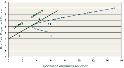
Since the risk-free asset is “risk-free”, it has zero variance. When adding the risk-free asset to the graph (assuming a risk-free rate of 3%), additional investment options become available that are more appealing than simply investing in Stocks A and B alone.

As you can see, to achieve the 6% expected return you are looking for, you’d be better off borrowing at the risk free rate and increasing the amount invested in the minimum variance portfolio (this scenario is represented by letter a on the graph) than you would be investing in the mixture of Stocks A and B represented by dot 11.
If you are more risk-adverse, buying the risk-free asset allows you to lower your standard deviation without forcing you to invest in a non-efficient portfolio. You could achieve a standard deviation of 2% while still earning a 4% expected return by lending some of your money at the risk-free rate and investing the rest in the minimum variance portfolio (see letter b on the graph).
Conclusion
Now, I know this article was a bit complicated and you’re probably thinking, “Mad Fientist, all this theory is great but now I don’t want to invest in the market at all because it seems too difficult. How do I know which stocks to buy? How can I borrow and lend at the risk-free rate?”
I understand your concerns. Next time, in the final article of this series, it will all become clear and I promise, the practical application of all of this theory is incredibly simple. In fact, my conclusions will most likely be similar to investment advice you have heard many times before. The only difference is, now you’ll have a better understanding of the financial theory supporting the advice and may feel more confident to act on it.
If you have any questions about what has already been covered, feel free to ask in the comments. Otherwise, give that calculator of yours a much needed rest and I’ll see you next time for the grand finale of the Unique Risk series!
Next article in the Unique Risk series: Market Portfolio


Insanely great blog you got going here. Much appreciated and thanks for the effort put into it!
Thanks a lot, Geronimo!
hey very nice article! may i ask how do you create the two graphs in this article? would help me greatly in my project. thanks!
Glad you enjoyed it, Barry.
I just used Excel to create the graphs and then I used Gimp to draw the risk-free asset line (I think).
Dear Mad FIentist,
Can you please elaborate on “…[borrowing] money at the risk-free rate by selling the risk-free asset and …[using] that extra money to invest more in the minimum variance portfolio.”
I think that I understand the leveraging implied here, but the source of the risk-free asset is not clear (to me); how does one borrow at 3%. Is the assumption that cash at-hand is earning 3% in a savings or money market account?
Thanks for the insightful blog posts and enlightening interviews. Your blogs have become a regular part of my quest for financial independence.
Kind regards,
Brunelleschi
Hi Brunelleschi,
Sorry for the delayed reply; I’ve been out of town and only returned late last night.
You are correct that borrowing implies leverage and in practice, you will likely not be able to borrow at the risk-free rate.
Using leverage to increase returns is not something I’d actually recommend doing so I’d instead suggest just owning the market (by purchasing a low-fee, broad-based index fund) and accepting the risk and returns that accompany investing in the stock market.
If you are more risk-averse, however, and would still like to invest in the market portfolio but want to reduce your risk, you could always use some of your money to lend at something close to the risk-free rate by buying bonds (buying a bond is effectively lending money to the bond issuer).
I’m glad you’ve been enjoying the blog and the podcast. Thanks a lot for the question!
Why would you not recommend using leverage to increase returns in real life? I know it sounds like a bad idea, but given that the math recommends it I’m having a hard time seeing why it really is one. Where does this theory break down in real life?
The closest part of it breaking down I can think of is that the risk-free borrowing rate is more than the risk-free lending rate (if you want to borrow money you pay a larger rate than you earn if you want to put money in a savings account). However, that seems like it would just mean that the efficient frontier would be the line from the risk-free lending rate to its tangency point, along the Markowitz bullet to the tangency point of the risk-free borrowing rate, and then along the risk-free borrowing rate line. Depending on where you look, you can borrow money at a lower rate than the market returns, so this difference between math and reality isn’t really a problem. What is?
Good stuff. Simplified and explained.
The question I have is on how do you determine (based on X), which stock to go with 75% and which with 25%. There is a contradiction in one of the above para””graphs – I have quote it below. Please clarify.
” For these two assets, investing 25% in Stock A and 75% in Stock B would allow you to nearly achieve a minimum variance portfolio for these two assets.
If we want to find the exact minimum variance portfolio allocation for these two assets, we can use the following equation:
x = (σb²-ρabσaσb) / (σa² + σb² – 2ρabσaσb)
Plugging in the values from the first article in this series, we can see that x = 74.42%. This means, to achieve a minimum variance portfolio that is invested in Stocks A and B, you should invest 74.42% in Stock A and 25.58% in Stock B.
Good evening,
I have a question: how do you calculate the fractions of the stocks composing your PF in the MVP with 3 stocks ?
Thank you
S.P
This is a great introductory series. Question: did personal capital get rid of their efficient frontier graph? I can’t seem to find it.
Great post. Could you explain how to quantify how much to borrow from the risk free rate in order to bring the 75/25% portfolio with expected return of 5% to match the 50/50% return represented by point 11?
Hi Madfientiest
Firstly thank you for your help (you’re making finance a lot easier for me).
Secondly, is it possible to explain how diversification helps with regards to the efficient frontier and Capital market/allocation line. (I understand how diversification eliminates idiosyncratic risk). I just don’t understand diversification in relation to portfolios and with regards to the efficient frontier and capital market allocation line.
I hope what I said makes sense.
Dis you ever find this answer S.D? My question is the same.
Fantastic explanation, just what I needed for my school assignment. Thanks man.